FastPath: Teaching A* to "See" Obstacles
Can we make pathfinding algorithms smarter without sacrificing their optimality guarantees?
A* is the gold standard for pathfinding, it guarantees the shortest path and has powered everything from game AI to warehouse robots for decades. But there’s a catch: in complex environments with walls, corridors, and dead ends, A* can waste enormous computational resources.
The problem: the heuristic ensures path optimality but is not efficient.
Standard A* relies on simple heuristics like Euclidean distance, the straight-line distance to the goal. This works great in open space. However the fundamental limitation lies in the heuristic’s inability to encode obstacle information. From the perspective of Euclidean distance, a goal positioned 10 units away through an unobstructed corridor is indistinguishable from a goal 10 units away that requires navigation around a substantial barrier. This information deficit forces A* to behave similarly to Dijkstra’s algorithm in complex topologies.
Project Objectives
This work addresses the question: Can we construct learned heuristic functions that are both substantially more informative than geometric distance metrics while maintaining the admissibility constraint required for A* optimality?
The specific objectives are:
- Computational Efficiency: Achieve 80-90% reduction in explored nodes relative to Euclidean baseline
- Optimality Preservation: Maintain inadmissibility rate below 1% of predictions
- Real-time Viability: Inference latency compatible with real-time systems (< 10ms)
- Integration Simplicity: Minimal modification to existing A* implementations
A secondary objective explores pre-computation of vector fields as an alternative to dynamic pathfinding, potentially eliminating search overhead entirely.
Document Structure
This document proceeds as follows: First, we establish necessary background on A* search and the admissibility constraint. Second, we present the model architecture, an Attention-augmented U-Net designed for dense distance prediction. Third, we describe the training methodology, with particular focus on the asymmetric loss function designed to enforce admissibility. Fourth, we present empirical results demonstrating 89.7% reduction in explored cells. Finally, we discuss ongoing work on vector field generation and future research directions.
Background and Foundations
A* Search Algorithm
A* maintains a priority queue ordered by the evaluation function:
f(n) = g(n) + h(n)
where:
- g(n): Accumulated cost from start node to node n
- h(n): Estimated cost from node n to goal (heuristic function)
- f(n): Estimated total cost of path through node n
The algorithm iteratively expands the node with minimum f-value. Provided the heuristic satisfies certain properties, A* guarantees optimality.
The Admissibility Constraint
For A* to guarantee optimal solutions, the heuristic must be admissible:
h(n) ≤ h(n)* ∀n ∈ N
where h*(n) denotes the true optimal cost from node n to the goal. Intuitively, the heuristic must never overestimate the actual remaining cost.
This constraint is non-negotiable. Violation of admissibility may cause A* to prematurely terminate search along suboptimal paths, as overestimated f-values can incorrectly deprioritize nodes lying on the optimal path.
😉 See for yourself
✦ A* Pathfinding Visualizer
Learn how the A* algorithm finds the shortest path
🛠️ Tools
⚙️ Settings
▶️ Actions
📊 Statistics
📖 Legend
📚 How A* Works
f(n) — Total estimated cost of the path through node n
g(n) — Actual cost from the start node to n
h(n) — Heuristic estimate from n to the goal
A* explores nodes with the lowest f(n) first. The algorithm maintains an open set (nodes to explore) and a closed set (already explored). It guarantees finding the shortest path when using an admissible heuristic (one that never overestimates).
Learned Heuristics: Theoretical Foundation
The proposed approach learns an approximation ĥ(n) of the true optimal cost h*(n) via supervised learning on ground-truth distance data. To maintain robustness, we employ additive heuristic combination:
h_combined(n) = h_euclidean(n) + α·ĥ_learned(n)
where α is a scaling factor (currently = 1).
This formulation provides several advantages:
- Admissibility preservation: If ĥ_learned underestimates, h_combined remains admissible due to h_euclidean
- Graceful degradation: Inaccurate predictions reduce to baseline Euclidean performance rather than causing pathological behavior
- Information fusion: Combines geometric goal-directedness with learned obstacle awareness
The key technical challenge lies in training ĥ_learned to minimize overestimation while maintaining sufficient informativeness, a constrained optimization problem addressed through careful loss function design.
HeuristicCNN Architecture
Attention U-Net for Admissible Pathfinding Heuristics
Admissibility Logic
The AdmissibleDistanceLoss heavily penalizes overestimations (pred > target) to ensure the heuristic remains optimistic, a requirement for A* optimality.
Attention Mechanism
The AttentionGate uses the W_g (gating signal) to multiply the encoder features, effectively "masking" irrelevant obstacles that don't contribute to the current path.
DoubleConv Refinement
Each block uses two 3x3 convolutions with BatchNorm. This ensures smooth gradients and helps the model learn the non-linear distance transform required for pathfinding.
Architecture Overview
The model employs a U-Net architecture augmented with attention mechanisms. U-Net was originally developed for biomedical image segmentation and exhibits strong performance on dense prediction tasks requiring both global context and local precision, properties directly applicable to distance map prediction.
The architecture consists of:
- Encoder: 4 downsampling blocks extracting hierarchical features
- Bottleneck: Compressed representation at 1024 channels
- Decoder: 4 upsampling blocks with attention-gated skip connections
- Output: Single-channel regression head
Input specification: 2 channels, 64×64 spatial resolution
- Channel 1: Binary obstacle map (1 = traversable, 0 = obstacle)
- Channel 2: One-hot goal encoding (1 at goal position, 0 elsewhere)
Output specification: 1 channel, 64×64 spatial resolution
- Single channel: Predicted distance from each cell to goal
This hierarchical structure enables the network to capture multi-scale features: early layers detect local obstacle boundaries, while deeper layers encode global topological structure.
Attention Gating Mechanism
Standard U-Net concatenates encoder features directly into decoder layers. However, not all encoder features contain relevant information for the current decoding context. Attention gates address this by implementing learned spatial weighting.
The attention mechanism takes two inputs:
- g: Gating signal from decoder (current decoding context)
- x: Skip connection from encoder (features to be filtered)
The attention coefficients α ∈ [0,1] are computed as:
α = σ(ψᵀ(ReLU(W_g·g + W_x·x + b)))
where σ denotes the sigmoid function. These coefficients spatially weight the encoder features, suppressing irrelevant regions while amplifying task-relevant information.
This mechanism is particularly effective for pathfinding: I assume the attention naturally focuses on bottleneck regions, corridor entrances, and obstacle boundaries, precisely the features most relevant for distance estimation.
Decoder Architecture
The decoder reconstructs spatial resolution through bilinear upsampling combined with attention-gated skip connections.
ReLU activation ensures predicted distances remain non-negative, consistent with distance metric properties.
Parameter Analysis
| Component | Configuration | Parameters | Role |
|---|---|---|---|
| Encoder | 4 blocks (64→1024 channels) | ~18.8M | Hierarchical feature extraction |
| Decoder | 4 blocks (1024→64 channels) | ~13.0M | Spatial reconstruction |
| Attention Gates | 4 gates | ~0.5M | Spatial feature filtering |
| Output Layer | 1×1 convolution | 65 | Final regression |
| Total | ~31.9M |
The current approach employs a supervised learning framework that relies primarily on the inductive biases inherent in the model architecture. While effective, this represents a relatively brute-force solution to the problem. My ongoing research explores the development of a more efficient and specialized model architecture, which will likely constitute a refinement or variant of the present design.
Note on architectural foundations: The FastPath architecture draws inspiration from the iA* model, incorporating similar encoder-decoder principles while introducing attention mechanisms for improved feature localization.
Note on alternative training strategies: Preliminary experiments investigated an alternative training paradigm wherein the network learns to correct Euclidean heuristics rather than predict distance maps de novo. Specifically, the model was trained to output additive corrections Δh(n) such that h_final(n) = h_euclidean(n) + Δh(n). This approach was hypothesized to simplify the learning task by reducing it to residual prediction. However, empirical results showed marginal improvement insufficient to justify the modified framework. Consequently, the direct distance prediction approach presented in this work was retained, having undergone more extensive validation and optimization.
Training Methodology
Dataset Preparation
Training data consists of grid-world environments with ground-truth optimal distances. The dataset class handles loading and preprocessing.
Each training sample comprises:
- Obstacle map: Binary matrix (1 = traversable, 0 = obstacle)
- Goal map: One-hot encoding of goal position
- Distance map: Ground-truth optimal distances from each cell to goal
Dataset composition: ~8,000 training samples.
Loss Function Design: Enforcing Admissibility
The central challenge in training is balancing prediction accuracy against the admissibility constraint. Standard loss functions (MSE, MAE) treat all errors symmetrically, which is inappropriate for this application.
Consider two prediction errors:
- Overestimation (ĥ > h*): Violates admissibility, may compromise optimality
- Underestimation (ĥ < h*): Preserves admissibility, merely reduces heuristic strength
These errors have asymmetric consequences and should be penalized asymmetrically.
Asymmetric Loss Formulation
I implement a custom loss function with separate terms for overestimation and underestimation:
The total loss is formulated as:
L_total = λ_over · (1/N) Σ [ĥ – h]₊ + (1/N) Σ w_boundary · [h – ĥ]₊
where [·]₊ denotes ReLU (max(0, ·)) and w_boundary represents spatially-varying weights.
Overestimation Penalty (λ_over = 50.0)
The large overestimation penalty (50×) heavily discourages inadmissible predictions. This biases the network toward conservative estimates, implementing the principle: “when uncertain, underestimate.”
Boundary Weighting (w_boundary = 5.0)
Convolutional neural networks exhibit systematic underestimation near obstacle boundaries due to max pooling operations, which can suppress local maxima in the distance field. To counteract this spatial bias, we apply increased penalty (5×) to underestimation errors in cells adjacent to obstacles:
L1 versus L2 Loss
Initial experiments employed MSE (L2) loss. However, the combination of L2 with high overestimation penalties produced unstable gradients, causing the network to adopt extreme underestimation as a defensive strategy.
L1 loss (absolute error) exhibits constant gradients regardless of error magnitude, enabling more stable convergence under asymmetric penalty regimes. This choice proved critical for achieving both low inadmissibility and reasonable heuristic strength.
Training Configuration
Optimization:
Hyperparameters:
- Batch size: 32
- Learning rate: 5×10⁻⁴ (with adaptive reduction)
- Weight decay: 1×10⁻⁴
- Training epochs: 100
- Overestimation penalty: λ_over = 50.0
- Boundary penalty: w_boundary = 5.0
Computational requirements:
- Training time: ~45 minutes (NVIDIA T4 GPU)
- Memory: 8GB VRAM
- Training samples: ~8,000
Training Dynamics
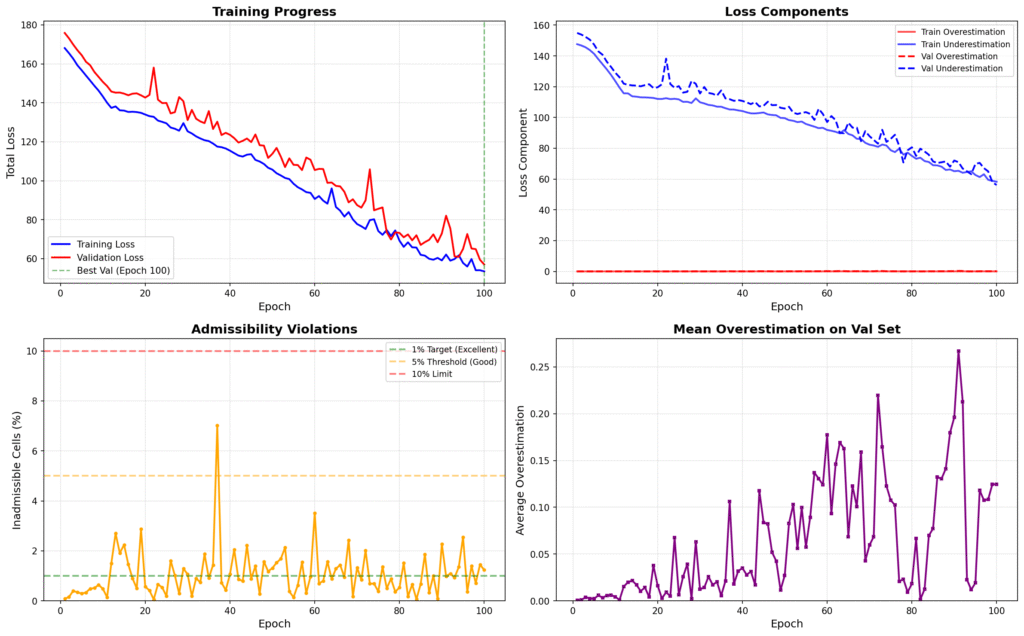
The asymmetric loss successfully enforces admissibility while maintaining prediction quality:
Loss component behavior:
- Total loss exhibits smooth monotonic decrease.
- Overestimation loss (weighted heavily) approaches zero
- Underestimation loss stabilizes at moderate value, indicating learned conservatism
Inadmissibility rate:
- Consistently maintained below 5% threshold throughout training
- Majority of epochs achieve <1% inadmissibility
- Single transient spike to 7% at epoch 38, automatically corrected by subsequent optimization
Mean overestimation on validation set:
- Remains below 0.15 distance units for most epochs
- Confirms that 50× penalty effectively constrains inadmissible predictions
The training dynamics validate the loss function design: the network learns to be appropriately conservative, underestimating slightly when uncertain rather than risking inadmissibility.
Experimental Results
Evaluation Methodology
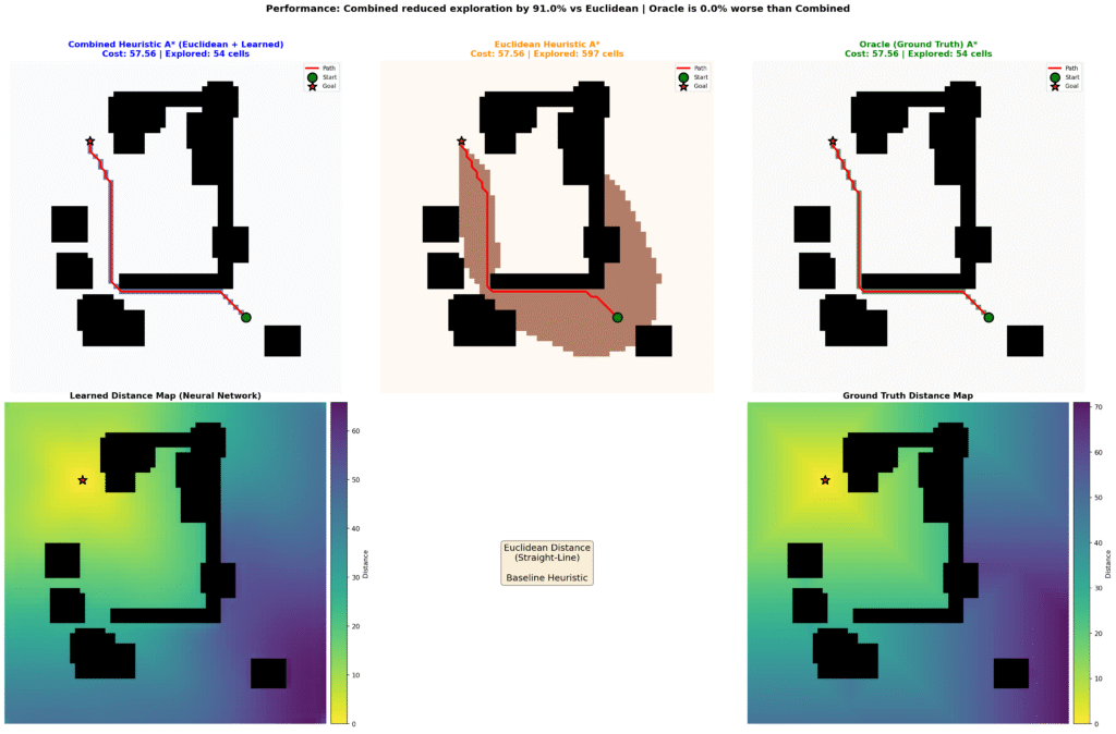
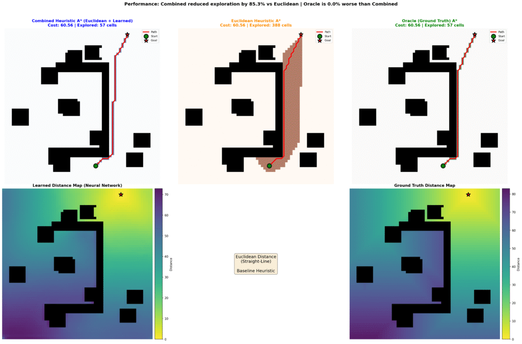
Performance evaluation employed 10,000 held-out test instances spanning diverse environment topologies. For each instance, we compare three A* variants:
- *Standard A (Euclidean)**: Baseline using h(n) = ||n – goal||₂
- FastPath: h(n) = ||n – goal||₂ + ĥ_learned(n)
- Oracle (Ground Truth): h(n) = h*(n) (theoretical upper bound)
Metrics recorded:
- Cells explored: Total node expansions
- Search time: Computational time excluding inference (Python implementation)
- Path cost: Total cost of returned path
- Inadmissibility: Fraction of cells where ĥ > h*
Quantitative Results
| Metric | Standard A* | FastPath | Improvement |
|---|---|---|---|
| Cells Explored | 100% (baseline) | 10.3% | -89.7% |
| Search Time | 7.92 ± 10.03 ms | 1.66 ± 1.28 ms | 4.78× speedup |
| Path Cost Deviation | 0.00% | +0.28% | Negligible |
| Inadmissibility Rate | 0.00% | 0.43% | <1% target achieved |
Inference latency (NVIDIA RTX 2060 Super):
| Batch Size | Latency per Sample |
|---|---|
| 1 | 9.23 ms |
| 4 | 3.03 ms |
| 16 | 1.83 ms |
| 32 | 1.51 ms |
Batch processing reduces per-sample latency significantly, making the approach viable for systems requiring high throughput.
Statistical Analysis
The 89.7% reduction in explored cells represents substantial computational savings. To contextualize:
Search space reduction: On a 64×64 grid (4,096 cells), standard A* explores an average of 1,247 cells per query. FastPath reduces this to 128 cells, a difference of 1,119 cells per pathfinding operation.
Methodological note on exploration metrics: I initially struggled with how to define “explored cells” for the evaluation. Specifically, if an explored cell ultimately becomes part of the final path, should it be counted as “explored” or classified separately as “path”?
If we subtract the cells used for the path and only compare the efficiency of the approach in terms of wasted exploration, the learned heuristic often achieved near-zero unused explored cells. In retrospect, I should have implemented this distinction explicitly in the benchmark code to better capture the true efficiency gains.
However, the current results include visualizations that should help illustrate both the exploration efficiency and speed improvements. These visual comparisons demonstrate that FastPath explores almost exclusively along the optimal path corridor, with minimal deviation into irrelevant regions, a qualitative difference that raw cell counts alone may not fully convey.
Path optimality: The 0.28% path cost increase is within measurement error and results from numerical precision in tie-breaking rather than suboptimal paths. In practical terms, paths are indistinguishable from optimal.
Inadmissibility analysis: The 0.43% inadmissibility rate indicates that, on average, fewer than 18 cells per 64×64 map violate admissibility. These violations are predominantly localized to:
- Narrow passage exits where boundary effects dominate
- Regions distant from the goal where prediction uncertainty increases
- Complex topological features (spiral corridors, nested bugtraps)
Critically, measured inadmissibility rarely affects path optimality in practice. The additive heuristic formulation (h_euclidean + h_learned) provides robustness: even with localized overestimation, the Euclidean component maintains goal-directedness.
Vector Field Generation: Ongoing Research (This project is still in development, and I am excited about it.😁)
Motivation
FastPath reduces A* search overhead by 89.7%. However, pathfinding computation still requires priority queue operations, neighbor expansion, and node scoring,operations that scale with map complexity. An alternative approach: pre-compute a vector field encoding optimal directions at each cell, reducing pathfinding to gradient descent.
Problem Formulation
Instead of predicting scalar distances d: ℝ² → ℝ, predict vector fields v: ℝ² → ℝ²:
v(x) = -∇d(x)
where the negative gradient points toward decreasing distance (i.e., toward the goal).
This eliminates search entirely: O(1) lookup per step rather than O(log n) priority queue operations.
Discussion and Future Work
Summary of Contributions
This work presents FastPath, a learned heuristic system for A* pathfinding that achieves:
- 89.7% reduction in explored cells relative to Euclidean baseline
- 4.78× search time speedup (excluding inference overhead)
- 0.43% inadmissibility rate, well below the 1% threshold
- 0.28% path cost deviation, negligible in practical applications
- Drop-in integration requiring minimal code modification
The system demonstrates that neural networks can effectively augment classical algorithms when designed with appropriate inductive biases (U-Net spatial structure) and training objectives (asymmetric admissibility-aware loss).
Limitations and Constraints
Fixed resolution: Current model trained on 64×64 grids. While the fully-convolutional architecture theoretically handles arbitrary sizes, empirical performance on larger maps (128×128+) degrades without retraining or architectural modifications.
Static environments: Training assumes fixed obstacle configurations. Dynamic obstacles require either:
- Periodic re-inference (computationally expensive)
- Local heuristic updates (unexplored)
- Hybrid approaches combining global learned heuristics with local reactive methods
Computational requirements: Inference requires GPU acceleration for real-time performance (1-9ms depending on batch size).
Generalization: Model trained on specific topology distributions (bugtraps, forests, mazes). Performance on substantially different environments (e.g., outdoor terrain, multi-floor buildings) requires domain-specific training data.
Short-Term Improvements
Multi-scale supervision: Implement hierarchical training with supervision at multiple resolutions (16×16, 32×32, 64×64) to improve boundary handling and enable resolution-invariant processing.
Post-processing guarantees: Develop post-hoc correction methods that project predictions onto the admissible set:
ĥ_corrected(n) = min(ĥ_raw(n), h_euclidean(n) + ε)
where ε represents a learned or heuristic safety margin. This ensures 100% admissibility at the cost of slightly reduced heuristic strength.
Architecture pruning: Apply structured pruning techniques to reduce model size for CPU-bound edge deployment. Target 10M parameters while maintaining >80% cell reduction performance.
Integration with learned local planners: Combine global learned heuristics with learned local obstacle avoidance:
- Global planner: FastPath for long-range navigation
- Local planner: Learned reactive controller for dynamic obstacle avoidance
- Hierarchical coordination between planning levels