FastPath: learned heuristics for A*

Abstract

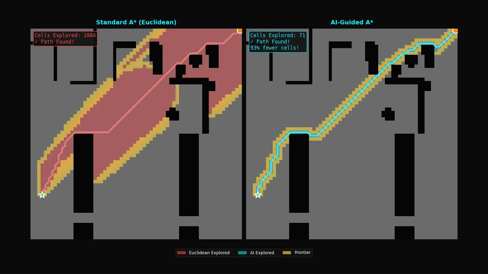
A* search guarantees the shortest path but struggles in cluttered maps because Euclidean distance ignores walls. FastPath trains an Attention U-Net model to predict an obstacle-aware distance map, adding it to the Euclidean baseline. This learned heuristic cuts the number of explored cells by 89.7% while increasing path cost by only 0.28%.

Introduction

Standard Euclidean distance pulls the search straight toward the goal. In environments with dead ends or bugtraps, this assumption fails and A* wastes time flooding the map.

• Maintain the guarantee. A heuristic that overestimates the distance breaks optimality. Admissibility must be trained for explicitly.
• Maintain the code. The solution must drop into an existing A* implementation without modifying the core priority queue.

The development sections below detail the network architecture, the asymmetric loss function, the integration step, and the performance results.

The model

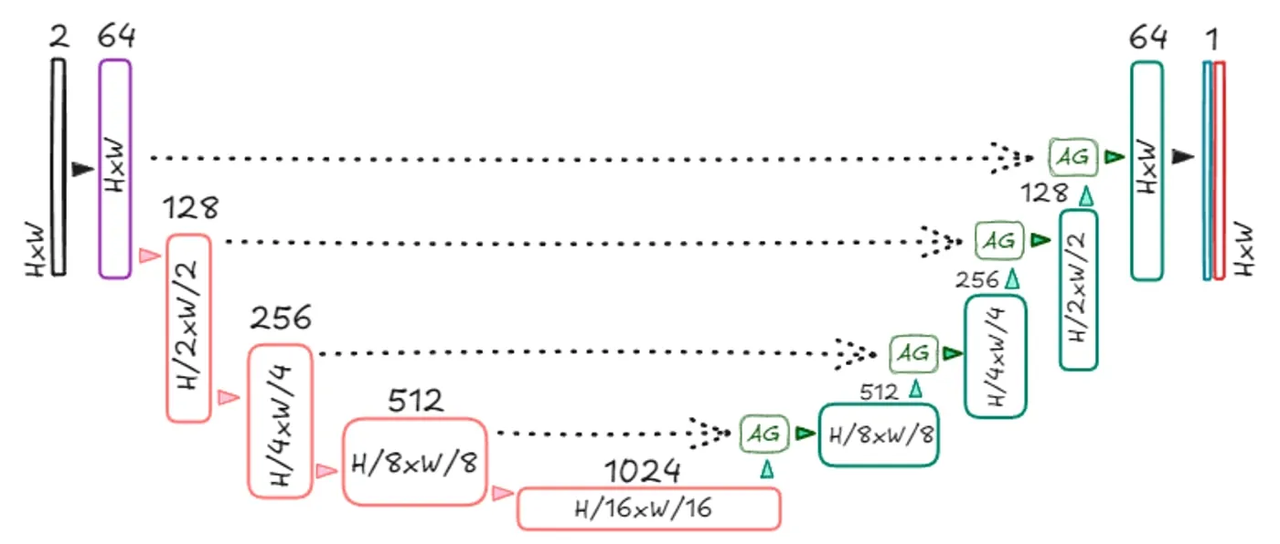
• Inputs. The model takes two 64x64 channels: a binary obstacle map and a one-hot goal location.
• Architecture. The encoder compresses from 64 to 1024 channels, and the decoder reconstructs the original resolution.
• Attention gates. These filter the skip connections to suppress empty open space while highlighting walls and bottlenecks.
• Outputs. A 1x1 convolution emits a single predicted distance value for every cell.

The loss

Admissibility is strictly asymmetric. Overestimating breaks optimality, while underestimating merely costs search speed.Toggle noteA* returns the optimal path as long as the heuristic never overestimates the true remaining cost.

$${ℒ}_{\text{total}}={\lambda }_{\text{over}}\cdot \frac{1}{N}\sum \text{ReLU}(h_{\text{pred}}-h_{\text{true}})+\frac{1}{N}\sum W_{\text{boundary}}\cdot \text{ReLU}(h_{\text{true}}-h_{\text{pred}})$$

• Asymmetric penalty (${\lambda }_{\text{over}}=50$). Overestimating the true cost is penalized 50 times harder than underestimating.
• L1 error. Using Mean Squared Error (MSE) with the huge penalty caused gradients to explode. The network learned to grossly underestimate everything, rendering it useless. L1 loss fixed this.
• Boundary weighting ($W_{\text{boundary}}=5.0$). Cells adjacent to walls carry 5 times the weight (1.0 elsewhere). Convolutions naturally blur transitions, but the heuristic needs sharp boundaries at walls.

Integration

One forward pass builds the entire distance map before the search begins. Every node evaluation after that is a simple array lookup.

$$h_{\text{combined}}(n)=h_{\text{Euclidean}}(n)+h_{\text{Learned}}(n)$$

def heuristic(pos):
    return euclidean(pos, goal) + learned_map[pos]

The combination is purely additive. The standard Euclidean term keeps pulling the search toward the goal even in areas where the network prediction is weak or perfectly flat.

Results

Metric	Euclidean A*	FastPath
Search time	7.92 ms	1.66 ms
Explored cells	100%	10.3%
Path cost	optimal	+0.28%
Inadmissible	0%	0.43%

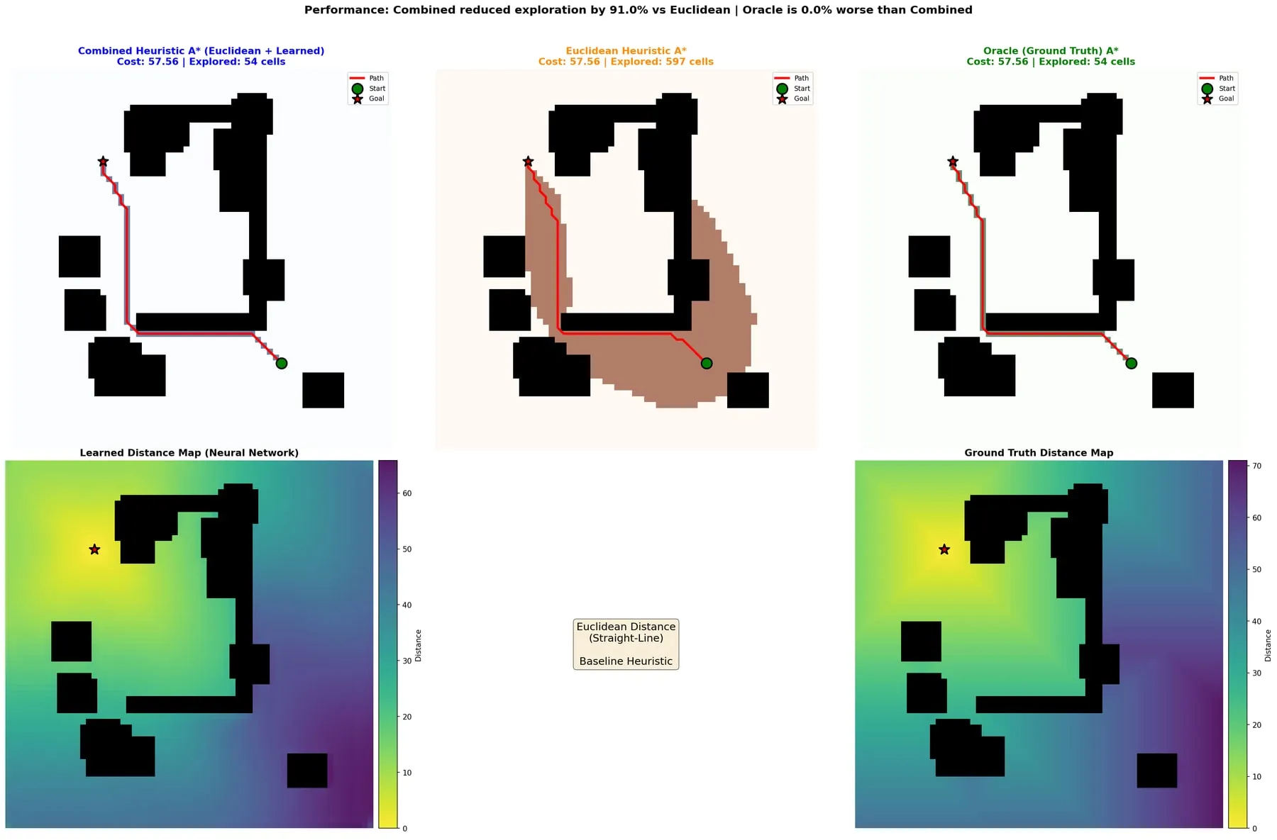
• Speed. FastPath searched 4.78 times faster over 10,000 randomized test instances.
• Accuracy. Paths remained nearly optimal, averaging just 0.28% longer than the true shortest path.
• Admissibility. The model overestimated on only 0.43% of cells, well below the 1% target.
• Training. The network trained in 35 minutes on an NVIDIA T4 using 3,200 samples. Inference takes just 1.51 ms per map.

Limits and next steps

• Fixed resolution. The network is hardcoded for 64x64 grids. Larger maps require tiling strategies or retraining.
• Static obstacles. Moving obstacles require full map re-inference or a separate local avoidance layer.
• Compute constraints. Inference runs best on a GPU. CPU-only edge devices would need an aggressively pruned model.